Probability Is the Engine: How Maths Powers Football Prediction Models
The Btcdices Team has spent time studying how stru


The Btcdices Team has spent time studying how structured predictive systems share the same foundational logic across wildly different domains. One of the clearest illustrations comes from the world of digital games: btc dices resolve every roll against a fixed, known probability distribution, with the expected return set against a house edge baked straight into the payout structure. Football prediction works from the same framework — but where dice games fix those probabilities in advance, a football model must estimate them from match data. That estimation process is where the real work begins, and it rests almost entirely on two tools: the Poisson distribution and expected value.
Turning Average Scoring Rates into Goal Probabilities
The Poisson distribution is a probability model built for exactly this kind of problem: estimating how likely it is that a given number of discrete events will occur within a fixed interval. A 90-minute football match fits that definition cleanly. Goals are discrete, they occur within a defined window, and the model can be fed a rate — an average number of goals a team scores or concedes — to produce a full probability curve across all possible tallies.
The inputs come from historical match data. Modellers typically draw on a team's average goals scored and average goals conceded across a season or a defined recent window, using those figures to construct a separate expected rate for each side in a given fixture. From there, the distribution calculates the probability of each team scoring zero goals, one goal, two goals, three, and so on.
A critical assumption sits underneath all of this: the Poisson model treats goals as independent events. One goal going in doesn't change the mathematical probability of the next. That's an approximation of reality rather than a perfect description of it, but it holds well enough across a large enough sample that it forms the basis of most quantitative football forecasting. Once you have a distribution for each team's likely tally, you combine the two independent distributions to generate probabilities for every possible scoreline — which then feeds every market a forecast might cover.
Shot Location, Shot Quality, and Why xG Matters
Raw goal tallies carry noise. A team that scores five goals in a week might have played brilliantly or might have converted a string of chances that, by any objective measure, were unlikely to go in. Over a small sample, the scoreline often tells you less than you'd hope about the underlying quality of the team's play.
Expected goals (xG) is the metric designed to cut through that noise. Each shot in a match receives a probability value based on factors including where on the pitch it was taken, the angle to goal, and the type of attempt. A tap-in from six yards carries a high xG value. A speculative strike from forty yards carries a very low one. Summing those values across all of a team's attempts gives a figure that reflects the quality of the chances they created, not just how many of them went in.
The practical payoff for prediction models is stability. A team's xG for and xG against, accumulated over a reasonable number of matches, provides a more reliable picture of their attacking and defensive quality than a goal tally would. Because actual goals are more susceptible to short-term variance, using xG as the input to a Poisson model produces rate estimates that are less likely to be distorted by a fortunate or unfortunate run of results.
Reading Bookmaker Odds Against a Model's Probability Estimates
Building a probability distribution is one thing. Knowing what to do with it requires one more concept: expected value. The calculation is straightforward in principle. You take the probability of an outcome, multiply it by the net payoff if that outcome occurs, and sum across all possible results. Positive expected value (EV) exists when your model's probability estimate for an outcome is higher than the probability the bookmaker's odds imply.
Bookmakers don't simply set odds to reflect their true probability estimates for each outcome. They build in a margin — called the overround or vigorish — so that the sum of all implied probabilities across a market's outcomes exceeds 100%. That excess is the house's mathematical edge, and it exists regardless of which result comes in. A prediction model only generates a meaningful edge when its probability estimate for a specific outcome sits clearly above the bookmaker's implied probability. The gap between those two figures is what defines the EV of a given position.
Over/under goals markets connect this logic directly back to the Poisson distribution. The probability of a match producing under 2.5 goals is simply the sum of the model's individual estimates for matches ending with zero goals, one goal, or two goals total. Once you have that cumulative figure, comparing it to the implied probability in the bookmaker's line tells you whether the market is priced in your favour. That's where the model's output becomes a practical tool rather than an academic exercise.
Football's High Variance and What It Means for Model Confidence
No part of understanding mathematical prediction is more important to get right than variance, and no sport makes variance more visible than football. Because goals are rare relative to higher-scoring sports, individual match results can diverge substantially from what a model's probabilities would suggest as the most likely outcome. An accurate model can identify a well-priced favourite and watch that favourite lose without a single shot on target. That's not a model failure. It's the probability distribution doing exactly what a probability distribution does.
The implication for sample size is direct. A team's xG and goal rate figures derived from a handful of matches are considerably less stable than the same metrics built across a full league season. The numbers shift too easily when the base is small. A full season of data allows the law of large numbers to work in the model's favour, pulling the estimates closer to the team's actual underlying quality and making the model's outputs more trustworthy as a result.
Accounting for this variance isn't a caveat bolted onto the end of a prediction model. It's built into the model's architecture from the start. A probability estimate is honest precisely because it doesn't claim certainty. It tells you how often a given outcome should occur if the same conditions repeated many times over. A model that presents its outputs as near-certain predictions isn't stronger than one that expresses appropriate uncertainty — it's just less truthful about what the mathematics actually says.